Working with the monthly export price of salmon

Abstract

We analyze the monthly export price of salmon time series which is available in the astsa package of R. The data set is called salmon in the package. The primary goal is to fit an appropriate SARIMA model to forecast future export prices and to gain a better understanding of the periodic behaviour of the series. From analyzing the ACF, I obtained evidence that the time series exhibits seasonal behaviour of 12 months. In the end, an ARIMA(1,1,0)x(0,1,1)[12] model was chosen. Then I forecasted into the future 10 months and found out that salmon prices increase overall in the next 10 months with a drop in price during the summer. From periodogram analysis, salmon export price has a dominant periodicity of 36 to 45 months. We have evidence that the export price of salmon has cyclical or periodic behaviour along with a seasonal pattern.

Introduction

There has been so much fluctuation in farmed salmon price over the years just like many other commodities in the market. Main reasons include biological interferences such as sea lice infestation and algal blooms. With rising demand in farmed salmon, farmers cannot just simply produce more salmon because they are faced with these biological interferences which may happen anytime. Other unwanted forces such as severe weather conditions and diseases also contribute to the volatility of salmon prices. So, one of the goals in this report is to deal with these random shocks by modeling with moving average and autoregressive components.

Additional research also shows that there is a growth cycle for salmon, which is they grow faster and eat more during certain times of the year. Specifically, Norwegian salmon fishing season is during the summer since the first weeks of June produces the biggest fish. Thus, we will fit a SARIMA model that will capture the seasonality aspect and random shocks of salmon prices. To do this, we will utilize the salmon data set available in the package astsa in R. The data is monthly export price of farm bred Norwegian salmon in US dollars per kilogram. A time series plot of this data is shown in Figure 1. As we can see, there is no obvious seasonal pattern, and this might be because the seasonality is masked by the high volatility of salmon price. The problem at hand will be to find the seasonality component in the SARIMA model with appropriate MA and AR components that will give us a reasonable forecast.

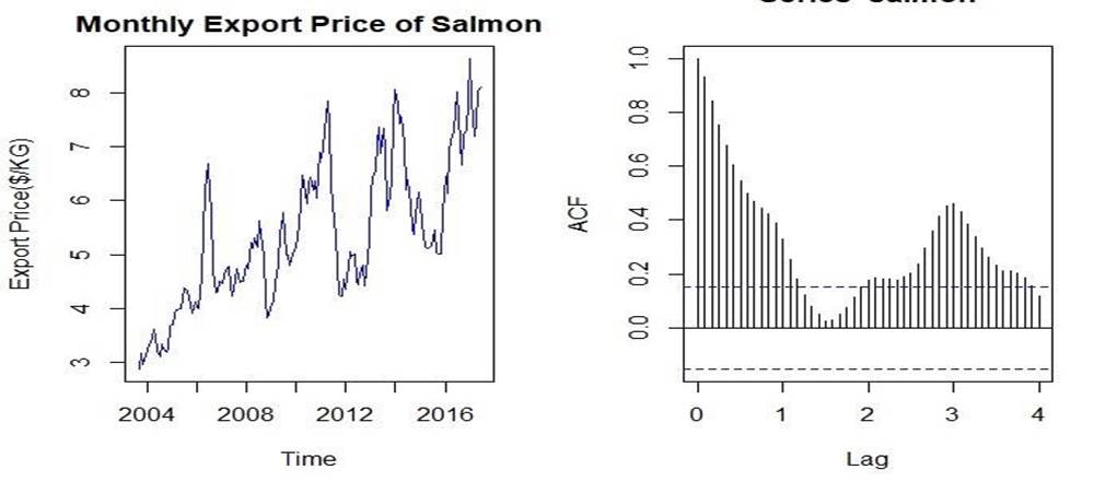
Figure 1

Exploratory Analysis

As shown by figure 1, there appears to be an upward trend in the export price of salmon series which needs to be removed by taking the first difference. Also, we can see from the ACF plot that the lag decays to 0 slowly which is an indication that differencing is needed.

Additionally, there appears to be some oscillation in the ACF which is indication of seasonality. After detrending the data by taking the first difference, I plotted the ACF of the first difference series (Figure 2) to show the seasonal component. We can see that there is significant lag every 6 months since the black line exceeds the blue dotted line. The significant peaks of the lag tend to occur every year and the significant troughs also repeats itself after a year. Since seasonal fluctuations occur every 12 months, a seasonal difference of 12 months should be applied in addition to an ordinary difference. We also gain evidence here to support our hypothesis that salmon prices indeed have yearly seasonal behaviour.

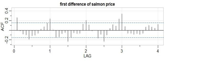
Figure 2

In total, I will apply a first ordinary difference to the salmon series to get rid of the trend, and then I apply a seasonal difference of 12 months because of seasonality shown in the above ACF plot. The final transformed series after taking the two differences is shown in Figure 3. The transformed series does not appear to have increasing variance, so we do not need any variance stabilization and overall, it looks approximately stationary. Now we are ready to identify the dependence orders for the SARIMA model using the ACF/PACF plot of this approximately stationary series.

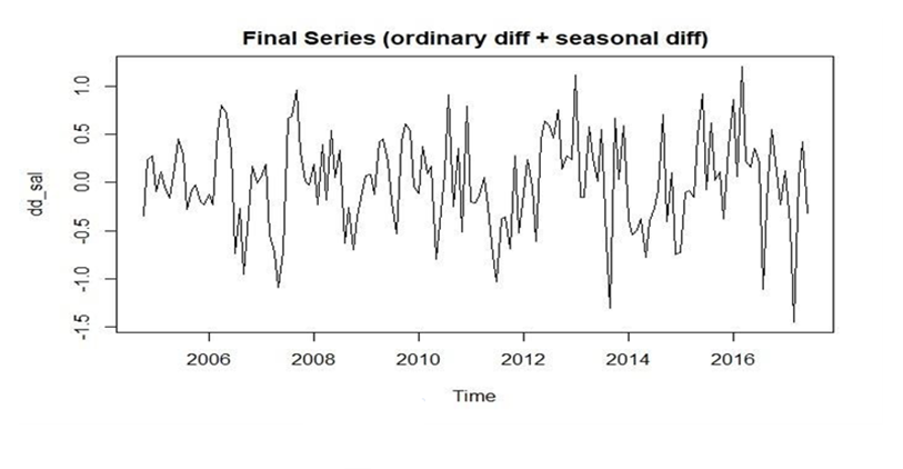
Figure 3

IDENTIFYING ORDERS OF SARIMA MODEL

We have previously defined d = 1 and D = 1. We took first ordinary difference (d = 1) and took a seasonal difference of S=12 months which is represented by D = 1. Now that preliminary values of d and D are chosen, we need to find (P, Q, p, q) by consulting the plot in Figure 4 below.

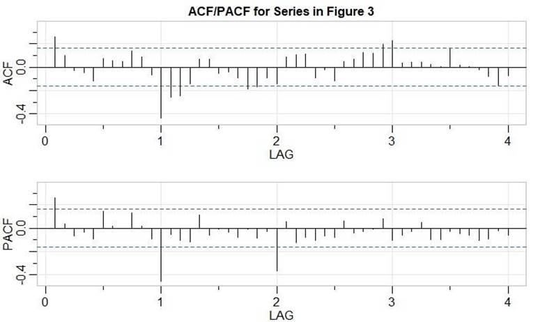
Figure 4

First Proposed Model: It appears that the ACF is cutting off at lag 12 which is 1*s where s = 12 and the PACF is tailing off at lags 12k (k = 1,2,3...). This implies a seasonal MA(1) model which means P = 0 and Q = 1. S = 12 as previously found. We see from the PACF at lower lags that there is a cut-off at lag 1. Also, from the ACF, there is a cut-off at lag 1. This means we can propose an AR(1) model or MA(1) model for the non-seasonal component. Since salmon prices are seasonal which means there is a period where the price is high and low afterwards, an AR(1) model would make more sense since previous prices have a direct effect on the future prices. We propose an AR(1) model for the non-seasonal component. This means p = 1 and q = 0. Together, we propose an ARIMA(p = 1, d = 1, q = 0) X (P = 0, D = 1, Q = 1)[S=12] model.

Second Proposed Model: It appears that the PACF cuts off at lag 24 which is 2*s where s = 12. The ACF is tailing off at lags 12k (k = 1,2,3...). This implies a seasonal AR(2) model which means P = 2 and Q = 0. For the non-seasonal component, before we proposed an AR(1) model since the PACF at lower lag cuts off at lag 1. Now we propose the alternative MA(1) model since it can also be argued that the ACF cuts off at lag 1. So, the second proposed model is ARIMA(p = 0, d = 1, q = 1) X (P = 2, D = 1, Q = 0)[S=12].

Fitting + Diagnosing the First Proposed Model: ARIMA(1,1,0)X(0,1,1)[12]

Parameter	Estimate	Standard Error	T value	P Value
Non-Seasonal AR1 (ar1)	0.2205	0.0791	2.7877	0.006
Seasonal MA1 (sma1)	-0.7958	0.0828	-9.6097	0.000

Table 1: Parameter estimates after fitting ARIMA(1,1,0)X(0,1,1)[12] on salmon price.

Interpretation and Estimates of Parameters:

From table 1, the AR parameter (ar1) estimate belonging to the non-seasonal part is 0.2205. The seasonal moving average (sma1) parameter estimate is -0.7958. We can interpret the sma1 parameter as follows; It is the size of the effect on the export price of salmon based on a shock that happened 12 months ago. For example, the sudden emerge of Covid-19 led to many fishing regulation and health concerns which may have affected salmon price a year later. We can think of the ar1 parameter to be the direct effect on salmon price based on the salmon price one month ago. The AR parameter estimate is 0.2205 which is a small direct effect on salmon export price based on salmon price one month ago. For example, if export price was X last month, the effect on the price this month is 0.2205X.

Testing the Significance of Parameter Estimates: The p values in table 1 for both the seasonal MA (sma1) and non-seasonal AR (ar1) parameters are very close to 0. It is less than the significance level of 0.05 so we reject the null hypothesis that the parameters are 0. We conclude that the parameter estimates are statistically significant.

Diagnostics: The diagnostic plot for the model is shown in Figure 5. The standardized residuals plot shows no obvious pattern which is indication of independent white noise and that our model fits well. However, there may be outliers exceeding 2 standard deviations in magnitude when what we want is the standardized residuals having magnitude around 1. The ACF plot of the standardized residuals show a significant spike at lag 28 but one is not enough to be significant at 5% level. There should be very little, if any, departure from the model assumption of uncorrelated residuals. From the normal QQ-plot, the assumption that the standardized residuals are normal is quite reasonable since there is little departure from the blue line. There are a few outliers near the tails from the QQ plot but overall, we can say the normality assumption is reasonable. We cannot claim the residuals are independent because the p value for L-Jung box statistic is significant at lag 36. Since lag 36 is a multiple of the seasonality of 12 months, there may be correlations that our model is not capturing. But our model is not supposed to be perfect anyway.

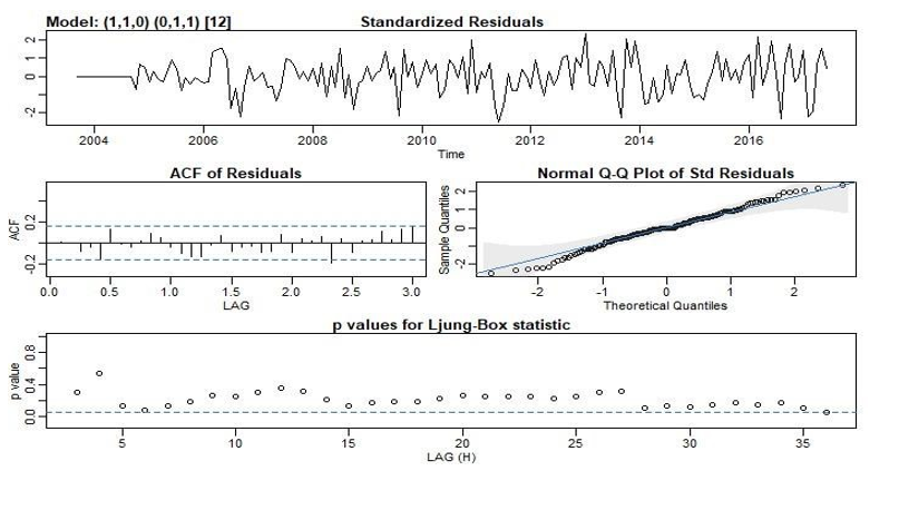
Figure 5

Fitting + Diagnosing the Second Proposed Model: ARIMA(0,1,1)X(2,1,0)[12]

Parameter	Estimate	Standard Error	T value	P Value
Non-seasonal MA1 (ma1)	0.1609	0.0761	2.1139	0.0362
Seasonal AR1 (sar1)	-0.6679	0.0745	-8.9648	0.0000
Seasonal AR2 (sar2)	-0.4837	0.0734	-6.5869	0.0000

Table 2: Parameter estimates and info after fitting ARIMA(0,1,1)X(2,1,0)[12]

Interpretation and Estimates of Parameters:

Table 2 gives the parameter estimates. The ma1 estimate can be interpreted as the size of the effect on the export price of salmon based on a shock that happened 1 month ago. In this case the "effect" is 0.1609 which is not that big. This is applicable to the export price of salmon because of natural phenomena. For example, natural disasters or new regulations on fishing may affect salmon price for a brief period of time and the effect gradually weakens. The seasonal AR1 and AR2 parameters play a role in determining the salmon price based on the salmon price 1 and 2 years ago. This may be unnecessary since salmon price too long ago may have no effect.

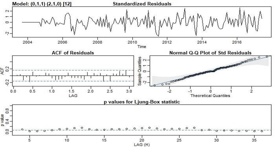
Figure 6

Diagnostics and Significance of Parameters:

From table 2, the p values are all below the significance level of 5% so we conclude that we have significant parameters. However, the p-values for L-Jung Box statistic in figure 6 above are almost all significant. This means we reject the null hypothesis that the residuals are independent. Since the residuals are not independent, this model may not be the best fit compared to our first model although the other diagnostic plots like normal QQ-plot looks fine.

Model Selection

The second model is more complicated since it has two seasonal AR parameters, but it also performs worse based on its p values in L-Jung Box statistic. It does not satisfy the model assumption because its p-values in L-Jung statistic is significant. So, its clear that we should choose the more parsimonious model, which is ARIMA(1,1,0)X(0,1,1)[12]. Now we forecast using this selected model.

Forecast Using Selected Model

Using ARIMA(1,1,0)X(0,1,1)[12], I will forecast the salmon export price in the next 10 months. A plot of the forecast of the salmon export price in next 10 months is given in Figure 7 below. Overall, salmon price is predicted to increase over the next 10 months with a price drop during the June summer period. The prediction intervals of the forecast are also increasing as time progresses which means there is more uncertainty of salmon price if we look far into the future. There are many reasons why the price is so unstable, such as sea lice, algal blooms and other biological factors that can interfere with health concerns. As a result, its hard to forecast salmon price too far into the future and hence the large prediction intervals. Prediction intervals are given in Table 3.

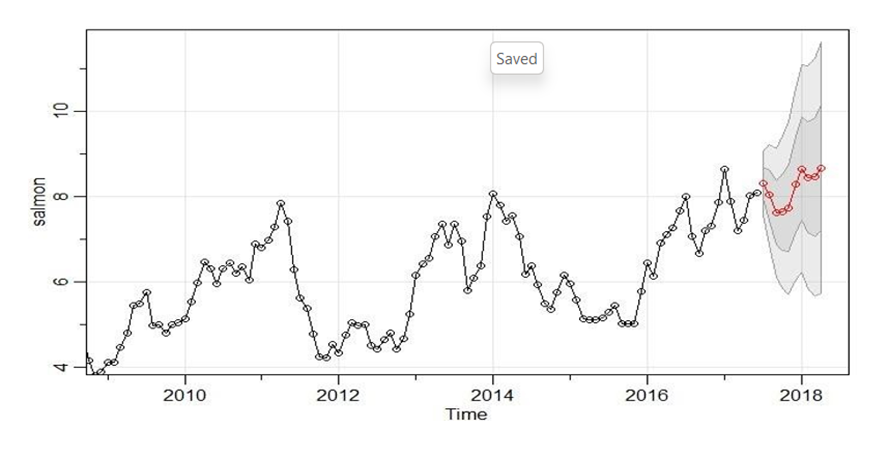
Figure 7

Future Week	Forecast	Lower Bound of PI	Upper Bound of PI
1	8.319999	7.590998	9.049001
2	8.036586	6.886329	9.186842
3	7.618651	6.142490	9.094812
4	7.637292	5.891085	9.383498
5	7.731674	5.751107	9.712241
6	8.283610	6.093459	10.473761
7	8.653043	6.271650	11.034436
8	8.454772	5.896386	11.013158
9	8.459431	5.735527	11.183335
10	8.671351	5.791426	11.551276

Table 3: Future 10 weeks forecast and its 95% prediction intervals

Spectral Analysis

We will now understand the periodic behaviour of salmon prices using spectral analysis. I performed a periodogram analysis and found that the first three predominant periods are 45 months, 36 months, and 12 months. Figure 8 shows the three dominant frequencies. The 95% confidence interval for the predominant period of 45 months is (0.4727, 68.8742) which is very wide so its hard to interpret. However, we see that the lower bound is 0.4727 which is higher than most other periodogram ordinate, so this peak is significant. We can also establish significance for the period of 36 months. Since the confidence interval for it is (0.3171, 46.2026), the lower bound of 0.3171 is higher than most other periodogram values so it is also significant. However, we cannot establish significance for the predominant period of 12 months. Its confidence interval is (0.1647, 23.99) which is wide in the first place. But unlike the other two confidence intervals, its lower bound is way too low to establish significance. Some other lower peaks are included in this interval because 0.1647 is not high enough to exclude them which means this peak is not significant. Combining the results, there appears to be a dominant periodicity of about 36 - 45 months since we were able to establish significance for those periods.

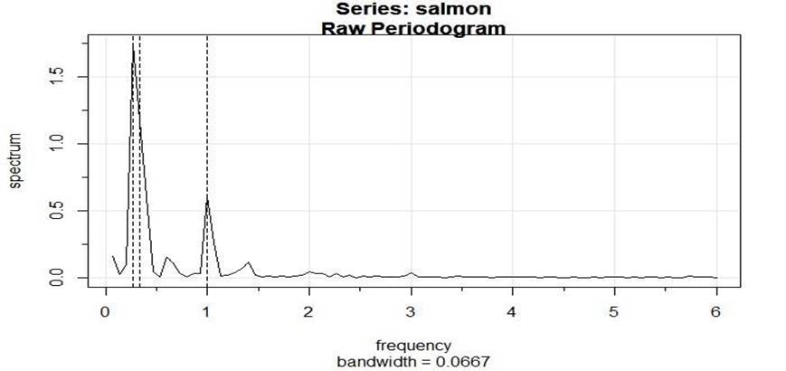
Figure 8

Discussion

As mentioned in the introduction, there is a yearly seasonal pattern in the price of salmon because Norwegian salmon are the biggest during the summer, so the supply chain is increased. We have evidence of this result as forecasting 10 months show that the price decreases over the summer period and goes back up when the next year begins. From spectral analysis, we also found that the salmon price has periodicity of about 3 to 4 years in addition to its seasonality. However, our model does have limitations because we observed the significant L-Jung p value at lag 36 in figure 5 and the normal QQ-plot has some outliers. This means our model is not capturing all the patterns of salmon price. There may be multiple seasonality that our model cannot capture because it requires more advanced models. For example, our model has seasonal lag of 12 because summer is the season for catching Norwegian salmon but there could be other seasonal patterns such as daily or monthly pattern that we are simply unaware about and which our model is not doing very well in capturing this relationship.